Tommi's Scribbles

Getting started analyzing AWS costs with Scala

Published on 2022-01-22
6 minute read

With so much happening in the cloud, keeping track of the costs associated with cloud services is key. AWS provides several tools to both estimate costs before committing, and monitoring costs after. In addition to the basic tools in the billing console, and the new dashboard that brings costs front and center, AWS also provides Cost and Usage Reports, or CURs. These reports allow fine-tuned granular analysis of your cloud costs. In this write-up, I show you a few examples what you can dig up from CURs with Scala.

Getting Started

First, one thing to note is that Cost and Usage Reports are not automatic. They have to be enabled in the billing console. Before this, no data is accumulated. Thus, it is important if you think you will utilize the reports, you enable them on your account as soon as possible. Otherwise, you will lose out on any trends you try to decipher.

As AWS has good documentation on enabling the CURs, I will not go through that here. One thing to note is that the guidance will promote using Athena for querying the data. This is not necessary. In fact, as the whole point is to try analyze costs, accumulating costs from the queries might not make a lot of sense. Especially since the data is your standard Parquet format, so you can easily use other tools to query the data. As the data resides in an S3 bucket, it is easy to create ETL flows outside of Athena as well.

Or, you can do as I did, and download the data for offline analysis. Once the data is on your computer, you can configure a Scala project. I did that using sbt and my favorite IDE with the Scala plugin. This is what the build.sbt looks like:

name := "cur-etl"

version := "0.1"

scalaVersion := "2.13.0"

idePackagePrefix := Some("com.company.cur")

libraryDependencies += "org.apache.spark" <><> "spark-core" <> "3.2.0"
libraryDependencies += "org.apache.spark" <><> "spark-sql" <> "3.2.0"
libraryDependencies += "org.apache.commons" <> "commons-csv" <> "1.8"

With the build config set up, we can start working on the actual scala file. We will start by configuring some libraries.

package com.company.cur

import org.apache.spark.sql.functions.{avg, col, greatest, lit, month, sum, year}
import org.apache.spark.sql.{DataFrame, SparkSession}

import java.io.{File, PrintWriter}
import scala.collection.mutable.ArrayBuffer
import scala.jdk.CollectionConverters._

Most of this is self explaining. We include some Spark query classes, basic file writing functionality, and some conversion helpers. Now we can start shaping up the actual code.

object cur {
val AllowedPriceDeviation = 1.33
def main(args: Array[String]): Unit = {
val spark: SparkSession = SparkSession.builder
.master("local[4]")
.appName("CUR")
.getOrCreate()
val df = spark.read.parquet("src/main/resources/")
.withColumn("year", year(col("line_item_usage_start_date")))
.withColumn("month", month(col("line_item_usage_start_date")))
.withColumn("max_cost", greatest("line_item_unblended_cost", "line_item_blended_cost"))
df.createOrReplaceTempView("cur")
findAnomaliesBetweenMonths(df, spark)
val printWriter = new PrintWriter(new File("output.csv"))
for (month <- 1 to 12) {
val monthlyData = buildDataForMonth(spark, month)
for (data <- monthlyData) {
printWriter.write(month.toString + "," + data)
}
}
printWriter.close()
spark.close()
}
}

We create an object named cur to house all our functionality. AllowedPriceDeviation is a helper value for later analysis. The main method is the cookie cutter standard main method that gets run.

The main method creates a SparkSession. I use local 4 to use all my physical cores, but you can pick e.g. 1 or 2 as well. If using a Spark cluster, you would use the cluster name here. I named my app creatively as "CUR"

Next, we read the downloaded CUR parquet files to a dataframe. Note the code expects you downloaded or copied the files to the src/main/resources folder. When creating the dataframe, we create a few extra columns to help group data: a year, a month, and a maximum cost of unblended and blended costs. Based on AWS documentation, either one is present depending if the cost is a discounted one or not. Hence, we want to pick the column with values.

We follow this by creating a view to the dataframe, again cleverly named as cur. Next, we call one of our ETL methods. The actual method code we will define later. That method will also demonstrate a different way of writing csv files.

We define a new print writer to write to a file named output.csv demonstrating an alternative way of exporting the data. The code then iterates through all the months, and calls another class method we will define later. We then output the monthly data to the csv file.

The main method is finished by closing the print writer stream and spark stream.

Highest cost items

With the main object and method fleshed out, we can move on to the actual bread and butter: the ETL methods. We start with the method we called from the main method: buildDataForMonth. The method will build top cost item data for each month, finding top 10 cost categories and involved resources for each month. As previously seen, the main method will then write the data to the output.csv for visualization.

def buildDataForMonth(spark: SparkSession, month: Int): ArrayBuffer[String] = {
val monthData = new ArrayBuffer[String](0)
val monthString = month.toString
val topCostDF = spark.sqlContext.sql("SELECT line_item_product_code AS service," +
"sum(max_cost) AS cost," +
"month FROM cur " +
"WHERE month='" + monthString + "' " +
"GROUP BY line_item_product_code, month " +
"ORDER BY cost DESC")
val topCostItems = topCostDF.takeAsList(10).asScala
for (item <- topCostItems) {
val itemCategory = item(0).toString
val itemsForMonth = findHighestCostItems(spark, itemCategory)
monthData.appendAll(itemsForMonth)
}
monthData
}

The code is pretty self-explanatory. There are a couple of different ways to query parquet data with Spark. Based on my research online, there is not much difference in which method to use. Here, we use the sqlContext.sql to query the data.

With the top 10 categoried collected, we then call another helper function to get all the resource IDs involved with the category using the method findHighestCostItems.

def findHighestCostItems(spark: SparkSession, itemCategory: String): ArrayBuffer[String] = {
val foundItems = new ArrayBuffer[String](0)
val itemDF = spark.sqlContext.sql("SELECT line_item_resource_id AS id," +
"line_item_operation," +
"line_item_usage_type," +
"sum(max_cost) AS cost FROM cur " +
"WHERE line_item_product_code='" + itemCategory + "' " +
"GROUP BY id, line_item_operation, line_item_usage_type " +
"ORDER BY cost DESC")
val items = itemDF.collectAsList().asScala
for (collectedItem <- items) {
foundItems.append(itemCategory + "," + collectedItem.mkString(",") + "\n")
}
foundItems
}

The code is again self-explanatory. With these two methods, we now get an output.csv with resources involved in the AWS top 10 cost accumulators for the particular data per month.

Deviations

In addition to the top 10 cost items, another item that can be tracked is finding anomalies: resources that suddenly experience a spike in cost above the average cost. We already saw the main method call this method: findAnomaliesBetweenMonths.

def findAnomaliesBetweenMonths(dataFrame: DataFrame, spark: SparkSession): Unit = {
val monthlyDF = dataFrame.groupBy("line_item_resource_id", "month")
.sum("max_cost")
.orderBy(col("line_item_resource_id"), col("month"))
val avgDF = monthlyDF.groupBy("line_item_resource_id")
.avg("sum(max_cost)")
val df = monthlyDF.join(avgDF, "line_item_resource_id")
.orderBy(col("line_item_resource_id"), col("month"))
val aboveAverageDF = df.filter(df("sum(max_cost)") > (lit(AllowedPriceDeviation) * df("avg(sum(max_cost))")))
aboveAverageDF.withColumn("deviation", aboveAverageDF("sum(max_cost)") / aboveAverageDF("avg(sum(max_cost))"))
.orderBy(col("deviation").desc)
.show(false)
aboveAverageDF.coalesce(1).write.option("header",true).csv("risks.csv")
}

The method again speaks for itself. We utilize the AllowedPriceDeviation we declared earlier to ignore small differences in the average costs. The code demonstrates another way of outputting the results as well: using coalesce to a CSV file.

Visualization examples using Tableau

We now have a simple local ETL (Extract, Transform, Load) Scala object we can run. The run produces us with two cleaned csv data files: one called output.csv housing all the top cost items and resources, and one in risks.csv housing resources that have had their costs increase.

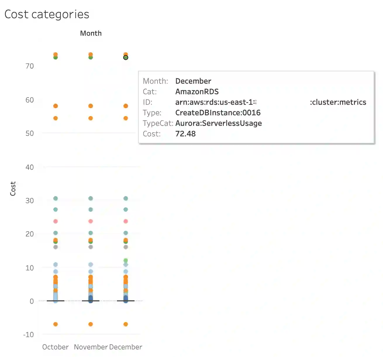
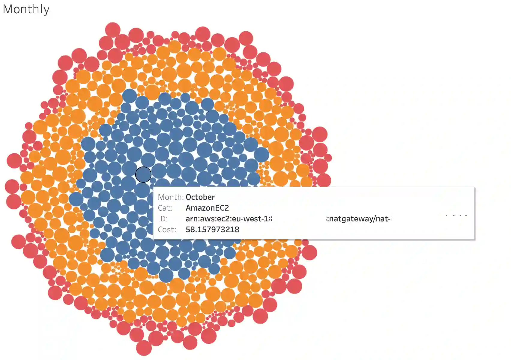
This data is ready for further analysis. For example, here is what the results can look like in Tableau. First, what the top 10 cost visualization could look like. A data visualization example showing charts And then, this is what the anomalies' visualization could look like.

Improvements

Obviously, we have just briefly touched the surface on how to use Scala to analyze AWS CURs (cost and usage reports). There are multiple different ways to go on about it depending on your needs, what insights you are looking to gain, and what tools you want to use.

The benefit of this method is that you get to sketch your ETL processes offline not accumulating costs from exploring the data, while still maintaining the ability to take your methods online, for example setting up clusters or creating an S3 triggered Lambda to create the cleaned data ready for analysis or monitoring from a different bucket.

The flexibility in exploring the data is also a benefit of tools such as Tableau and Power BI. Creating different visualizations, exploring drill-downs, finding insights, and learning what is important is easy. Once settled you can replicate the visualizations with something like Observable or Datalore to create automatically refreshing embeddable dashboards for anyone to use.